The Riparian Condition Assessment Toolbox can be run using either freely available national datasets (for the U.S.) or with higher resolution datasets.
Inputs
The Riparian Condition Assessment Toolbox (RCAT) requires the following input files:
- A polyline shapefile representing the stream network (see the National Hydrography Dataset for freely available U.S. stream flowlines)
- A digital elevation model (DEM) (see The National Map to download from the National Elevation Dataset)
- Existing and historic vegetation landcover rasters (see the LANDFIRE website for freely available U.S. vegetation data including the Existing Vegetation Type [existing vegetation] layer and Biopyhsical Settings [historic vegetation] layer)
- A precipitation raster (see the PRISM website for freely available U.S. precipitation data)
- If you want to account for dredge tailing impacts, download mine-related spatial data from the USGS Mineral Resources website for the state of interest. This shapefile will represent all mining activity in your watershed, so you will want to select the features representing dredge tailings and export these to a new shapefile.
For efficiency, the vegetation rasters, DEM, precipitation raster, and dredge tailings shapefile should be clipped to the watershed boundary. All data should also be projected to the same coordinate system to avoid errors.
Stream Network Preparation
- Prepare a stream network using the NHD Network Builder tool
- Dissolve and segment the network using the Segment Network tool. (~300 meter segments work well)
Vegetation Data Preparation
For both the historic and existing vegetation rasters, add and populate the following fields:
RIPARIAN(type = Short Integer): Binary field for riparian vegetation, including non-native riparian vegetation, classified as follows:0= Not riparian landcover1= Riparian landcover
NATIVE_RIP(type = Short Integer): Binary field for native riparian vegetation, classified as follows:0= Not native riparian landcover1= Native riparian landcover
CONVERSION(type = Short Integer: Landcover vegetation groupings, classified as follows:500= Open water100= Riparian65= Deciduous or hardwood upland forest50= Grassland or shrubland40= Non-vegetated, sparsely vegetated, snow/ice, sand, barren, etc.20= Conifer or conifer-hardwood forest3= Exotic, introduced, and invasive landcover2= Developed, including urban areas, roads, quarries or gravel pits, etc.1= Agriculture-9999= No data value for landcover classes that don’t fit into any of the above
VEGETATED(type = Short Integer): Binary field for any native vegetation, classified as follows:0= All non-vegetated areas or non-native vegetated landcover, including but not limited to open water, barren, snow/ice, developed, barren, exotic and introduced landcover, etc.1= All native vegetation landcover, including but not limited to native riparian, sagebrush steppe, conifer forest, conifer-hardwood forest, native grassland, native shrubland, etc.
LU_CODE(type = Double): Land use intensity code (only needed in existing vegetation raster), classified as follows:0= Very low land use or natural landcover, including nonnative vegetation0.33= Low land use, including low intensity agriculture such as fallow or idle cropland, pasture, and hayland0.66= Moderate land use, including high intensity agriculture such as aquaculture, bush fruit and berry agriculture, orchards, vineyards, close grown crops or row crops, wheatlands, and managed tree plantations1.0= High land use, including urban, quarries, strip mines, gravel pits, roads, and developed landcover of any form
NOTE: The Add LANDFIRE Fields tool will add and populate the
CONVERSION,VEGETATED, andLU_CODEfields to LANDFIRE datasets, but these fields should be double-checked since this code was developed using only the 2016 LANDFIRE remap for a limited styudy area, so some landcover classes may be missing.
Valley Bottom Preparation
One of the required inputs is a valley bottom polygon that has been fragmented using a transportation infrastructure network (roads, railroads, etc.). The following process describes how to derive this input:
- Produce a valley bottom using VBET, and manually edit to desired accuracy.
- Overlay a finalized road/railroad network on a copy of a final, edited valley bottom polygon.
NOTE: National road and railroad datasets can be found on the TIGER website.
- Begin editing the valley bottom polygon. Select the whole road/railroad network (right click on the shapefile, go to “Selection” and choose “Select All”).
- Go to “Editor” > “More Editing Tools” > “Advanced Editing”
- Click on the “Split Polygons” tool and split the valley bottom using the transportation network.
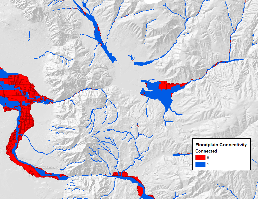
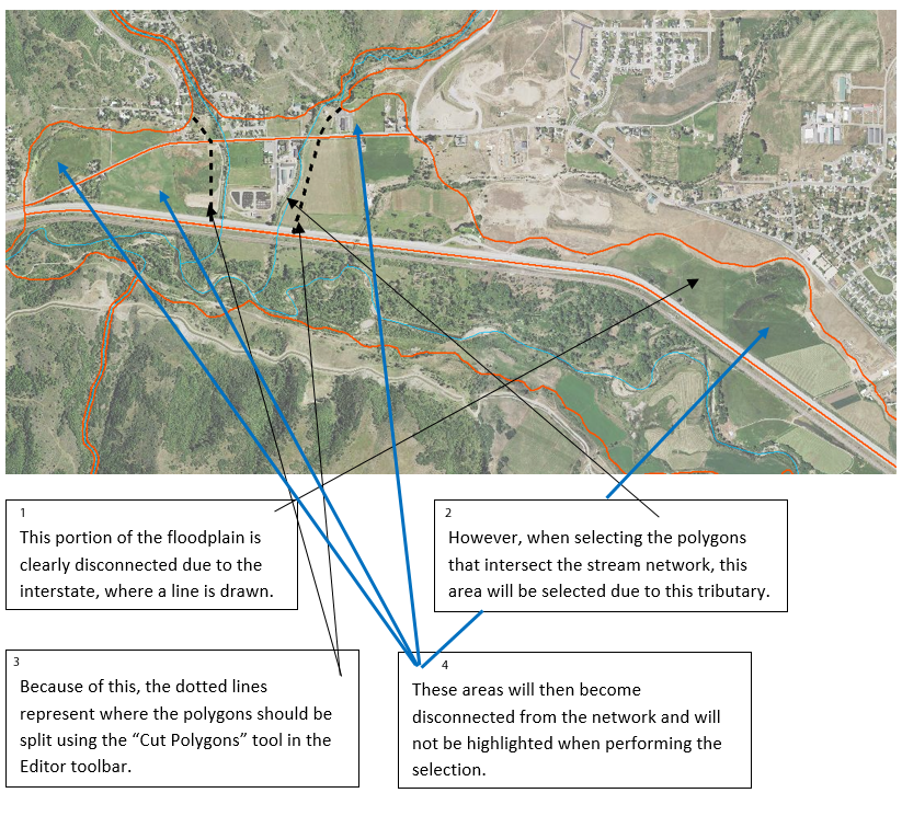
- Go through the split valley and manually fix polygons that need to be enclosed. (Areas where the stream does not intersect a polygon will be considered disconnected from the floodplain. See figure below.)
- Add a field (type = Short Integer) to the split valley bottom feature and name it “Connected”.
- Make sure you are still editing the split valley bottom.
- In “Select by Location” select the portions of the split valley bottom polygon that the stream network intersects. In the attribute table, change value of the “Connected” field to 1 for the highlighted features.
- All other features should have a value of 0. (If necessary, reverse the selection and give the now highlighted features a value of 0.)
- Export the feature as a new shapefile with a name referring to floodplain connectivity. This will be used as an input in the RCA tool.
The figure below shows a final split valley bottom, ready for use in the tool.